Modul 4 Praktikum Sains Data

Modul 4 Praktikum Sains Data

Outline

1. Review Evaluation Metrics pada Klasifikasi
2. Decission Tree
3. SVM

1. Evaluation Metrics

1. Jaccard Index

Mengukur akurasi dari model menggunakan irisan dari hasil prediksi dengan value sebenarnya. \[J(y, \hat{y}) = \frac{|y \cap \hat{y}|}{|y|+|\hat{y}|-|y \cap \hat{y}|}\]

\(y=\) actual label

\(\hat{y}=\) predicted label

Contoh:

\(y = [0,0,0,0,0,1,1,1,1,1]\)

\(\hat{y} = [1,1,0,0,0,1,1,1,1,1]\)

\(|y| = 10\)

\(|\hat{y}| = 10\)

\(|\hat{y}|-|y \cap \hat{y}| = 8\)

\(J(y, \hat{y}) = \frac{|y \cap \hat{y}|}{|y|+|\hat{y}|-|y \cap \hat{y}|} = \frac{8}{10+10-8} = 0.66\)

• Rentang Jaccard index antara 0 hingga 1
• Semakin tinggi Jaccard Index, peforma model semakin baik

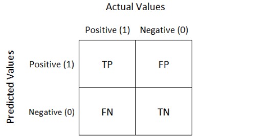
2. Confusion Matrix, F1 Score

TN / True Negative: kasus negatif, dengan hasil prediksi negatif

TP / True Positive: kasus positif, dengan hasil prediksi positif

FN / False Negative: kasus positif, dengan hasil prediksi negatif

FP / False Positive: kasus negatif, dengan hasil prediksi positif

\[Precision = \frac{TP}{(TP+FP)}\]

\[Recall = \frac{TN}{(TP+FN)}\]

\[F1 \text{ } Score = \frac{2 . (Recall.Precision)}{(Recall+Precision)}\]

Cara mengukur performa menggunakan F-1 score dengan mengambil rata rata F1-score dari masing masing label.

Contoh, label 0 memiliki F1-score 0.72 dan label 1 memiliki F1-score 0.50.

Maka, F1-score dari model tersebut adalah 0.61

• Rentang F1-score berkisar di antara 0 hingga 1
• Semakin tinggi F1-score, maka peforma model tersebut makin baik

3. Log loss

Terkadang, output dari suatu model klasifikasi berbentuk probabilitas dari suatu item memiliki label tertentu. (Contohnya pada logistic regression minggu lalu)

Kita dapat menghitung untuk masing-masing item: \[(y. \log(\hat{y}) + (1-y). \log(1-\hat{y}))\]

Kemudian, kita dapat menghitung rata rata dari tiap item tersebut \[Logloss = -\frac{1}{n} \Sigma (y. \log(\hat{y}) + (1-y). \log(1-\hat{y}))\]

\(y=\) actual label

\(\hat{y}=\) predicted probability

Contoh:

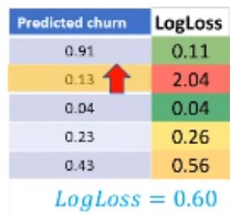
• Rentang logloss berkisar di antara 0 hingga 1
• Semakin rendah logloss, maka peforma model tersebut makin baik

2. Decision Tree

Seperti namanya, pohon keputusan, konsepnya bentuknya pohon, bercabang.

Biasanya digunakan sebagai simple binary classifier.

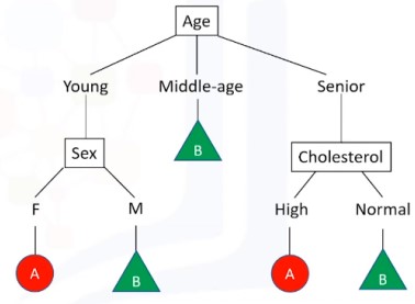
• Mencari fitur apa yg membuat suatu item memiliki label tertentu
• Entropy = tolak ukur seberapa random data di fitur tsb, entropy 0 artinya simpul (fitur) tsb berpengaruh terhadap klasifikasi, entropy 0 itu baik \[-P(A).\log(P(A)) - P(B).\log(P(B))\]
• Information gain : informasi yang dapat meningkatkan kejelasan dari percabangan. \(\newline\) InfoGain = Entropybefore - weightedentropyafter
• Pohon yg lebih baik adalah yang memiliki infogain lebih tinggi

Kali ini, kita akan mengklasifikasi resep obat yang cocok dari penyakit yang sama untuk fitur-fitur yang berbeda (Umur, Jenis Kelamin,Tekanan Darah, Kolestrol)

Import Module

#import modul dan package
import numpy as np
import pandas as pd
from sklearn.tree import DecisionTreeClassifier

Import Data

Pada module kali ini, akan digunakan data csv drug200 (drug200.csv) yang bisa didownload dari:

• Kaggle

#muat dataset
my_data = pd.read_csv(r".\drug200.csv")
my_data.head()

	Age	Sex	BP	Cholesterol	Na_to_K	Drug
0	23	F	HIGH	HIGH	25.355	drugY
1	47	M	LOW	HIGH	13.093	drugC
2	47	M	LOW	HIGH	10.114	drugC
3	28	F	NORMAL	HIGH	7.798	drugX
4	61	F	LOW	HIGH	18.043	drugY

my_data.shape

(200, 6)

#melihat ada brp value berbeda pada feature/kolom Drug
my_data["Drug"].unique()

array(['drugY', 'drugC', 'drugX', 'drugA', 'drugB'], dtype=object)

#feature/kolom pada dataframe
my_data.columns

Index(['Age', 'Sex', 'BP', 'Cholesterol', 'Na_to_K', 'Drug'], dtype='object')

#melihat value per baris
X = my_data[['Age', 'Sex', 'BP', 'Cholesterol', 'Na_to_K']].values
X[0:5]

array([[23, 'F', 'HIGH', 'HIGH', 25.355],
       [47, 'M', 'LOW', 'HIGH', 13.093],
       [47, 'M', 'LOW', 'HIGH', 10.114],
       [28, 'F', 'NORMAL', 'HIGH', 7.798],
       [61, 'F', 'LOW', 'HIGH', 18.043]], dtype=object)

Preprocessing

Pada bagian ini, kita akan mengubah value kategorik menjadi data numerik

from sklearn import preprocessing
le_sex = preprocessing.LabelEncoder()
le_sex.fit(['F', 'M'])
X[:, 1] = le_sex.transform(X[:, 1]) #sex di kolom kedua df, indexnya 1
X[0:5]

array([[23, 0, 'HIGH', 'HIGH', 25.355],
       [47, 1, 'LOW', 'HIGH', 13.093],
       [47, 1, 'LOW', 'HIGH', 10.114],
       [28, 0, 'NORMAL', 'HIGH', 7.798],
       [61, 0, 'LOW', 'HIGH', 18.043]], dtype=object)

le_bp = preprocessing.LabelEncoder()
le_bp.fit(['LOW', 'NORMAL', 'HIGH'])
X[:, 2] = le_bp.transform(X[:, 2]) #sex di kolom ketiga df, indexnya 2
le_chol = preprocessing.LabelEncoder()
le_chol.fit(['NORMAL', 'HIGH'])
X[:, 3] = le_chol.transform(X[:, 3]) #sex di kolom keempat df, indexnya 3
X[0:5]

array([[23, 0, 0, 0, 25.355],
       [47, 1, 1, 0, 13.093],
       [47, 1, 1, 0, 10.114],
       [28, 0, 2, 0, 7.798],
       [61, 0, 1, 0, 18.043]], dtype=object)

y = my_data['Drug']
y[0:5]

0    drugY
1    drugC
2    drugC
3    drugX
4    drugY
Name: Drug, dtype: object

Train/Test Split

from sklearn.model_selection import train_test_split
X_train, X_test, y_train, y_test = train_test_split(X, y, test_size = 0.3)

print(X_train.shape)
print(y_train.shape)

(140, 5)
(140,)

print(X_test.shape)
print(y_test.shape)

(60, 5)
(60,)

Modelling

from sklearn.tree import DecisionTreeClassifier

drugtree = DecisionTreeClassifier(criterion = 'entropy', max_depth = 4)

drugtree.fit(X_train, y_train)

DecisionTreeClassifier(criterion='entropy', max_depth=4)

In a Jupyter environment, please rerun this cell to show the HTML representation or trust the notebook.
On GitHub, the HTML representation is unable to render, please try loading this page with nbviewer.org.

predTree = drugtree.predict(X_test)
predTree

array(['drugC', 'drugY', 'drugX', 'drugY', 'drugX', 'drugX', 'drugY',
       'drugX', 'drugY', 'drugX', 'drugY', 'drugC', 'drugC', 'drugY',
       'drugB', 'drugX', 'drugA', 'drugY', 'drugY', 'drugC', 'drugX',
       'drugC', 'drugX', 'drugY', 'drugY', 'drugB', 'drugB', 'drugC',
       'drugY', 'drugY', 'drugY', 'drugY', 'drugC', 'drugY', 'drugY',
       'drugY', 'drugY', 'drugY', 'drugA', 'drugX', 'drugY', 'drugY',
       'drugY', 'drugB', 'drugY', 'drugY', 'drugA', 'drugA', 'drugX',
       'drugX', 'drugY', 'drugY', 'drugY', 'drugY', 'drugX', 'drugX',
       'drugX', 'drugA', 'drugY', 'drugA'], dtype=object)

#bandingkan nilai y pada data uji dengan hasil prediksi
comparison = {"y_test" : y_test,
              "Predicted": predTree}
comp = pd.DataFrame(comparison)
comp

	y_test	Predicted
10	drugC	drugC
90	drugY	drugY
132	drugX	drugX
23	drugY	drugY
145	drugX	drugX
34	drugX	drugX
154	drugY	drugY
37	drugX	drugX
49	drugY	drugY
58	drugX	drugX
123	drugY	drugY
47	drugC	drugC
195	drugC	drugC
121	drugY	drugY
108	drugB	drugB
135	drugX	drugX
61	drugA	drugA
24	drugY	drugY
157	drugY	drugY
84	drugC	drugC
181	drugX	drugX
102	drugC	drugC
45	drugX	drugX
19	drugY	drugY
125	drugY	drugY
142	drugB	drugB
41	drugB	drugB
2	drugC	drugC
166	drugY	drugY
94	drugY	drugY
28	drugY	drugY
9	drugY	drugY
193	drugC	drugC
74	drugY	drugY
164	drugY	drugY
91	drugY	drugY
115	drugY	drugY
88	drugY	drugY
36	drugA	drugA
160	drugX	drugX
172	drugY	drugY
48	drugY	drugY
22	drugY	drugY
136	drugB	drugB
62	drugY	drugY
165	drugY	drugY
140	drugA	drugA
100	drugA	drugA
81	drugX	drugX
159	drugX	drugX
75	drugY	drugY
0	drugY	drugY
29	drugY	drugY
12	drugY	drugY
63	drugX	drugX
182	drugX	drugX
105	drugX	drugX
176	drugA	drugA
33	drugY	drugY
174	drugA	drugA

Akurasi

from sklearn.metrics import accuracy_score
print("Accuracy : ", accuracy_score(y_test, predTree))

Accuracy :  1.0

Visualisasi Decision Tree

from sklearn import tree

featureNames = my_data.columns[0:5]

graph = tree.plot_tree(drugtree,
                       feature_names=featureNames,
                       class_names=np.unique(y_train),
                       filled=True)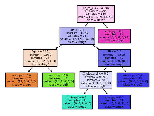

3. Support Vector Machine

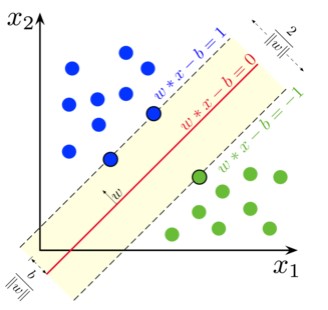
SVM adalah algoritma supervised learning utk klasifikasi dengan cara menemukan separator berupa hyperplane (biasanya utk binary classification)

1. Petakan fitur (kolom, bentuk awalnya 1d) ke ruang dimensi yg lebih tinggi (contohnya 3D) menggunakan fungsi kernel (linear, Radial Basis Function, polinom, sigmoid, dsb)
2. Temukan separatornya (utk di ruang 3d biasanya bentuknya bidang)

• Hyperplane yg baik adalah yg memiliki margin lebih besar (jarak ke support vector)

SVM

Kali ini, kita akan melakukan klasifikasi sebuah cell apakah cell tersebut jinak atau ganas (berpotensi kanker)

#install dulu package bila belum memiliki sklearn
!pip install scikit-learn==0.23.1

Import Module

#import modul yang diperlukan
import pandas as pd
import pylab as pl
import numpy as np
import scipy.optimize as opt
from sklearn import preprocessing
from sklearn.model_selection import train_test_split
%matplotlib inline
import matplotlib.pyplot as plt

Import Dataset

Pada module kali ini, akan digunakan data csv cell samples (cell_samples.csv) yang bisa didownload dari:

• Kaggle

#memuat dataframe
cell_df=pd.read_csv(r".\cell_samples.csv")

cell_df.head()

	ID	Clump	UnifSize	UnifShape	MargAdh	SingEpiSize	BareNuc	BlandChrom	NormNucl	Mit	Class
0	1000025	5	1	1	1	2	1	3	1	1	2
1	1002945	5	4	4	5	7	10	3	2	1	2
2	1015425	3	1	1	1	2	2	3	1	1	2
3	1016277	6	8	8	1	3	4	3	7	1	2
4	1017023	4	1	1	3	2	1	3	1	1	2

#melihat sebaran datanya menggunakan scatterplot
ax = cell_df[cell_df['Class']==4][0:50].plot(kind='scatter', x='Clump', y = 'UnifSize', color = 'Blue',
                                             label = 'ganas')
cell_df[cell_df['Class']==2][0:50].plot(kind='scatter', x='Clump', y = 'UnifSize', color = 'Yellow', 
                                        label ='jinak',ax=ax)
plt.show()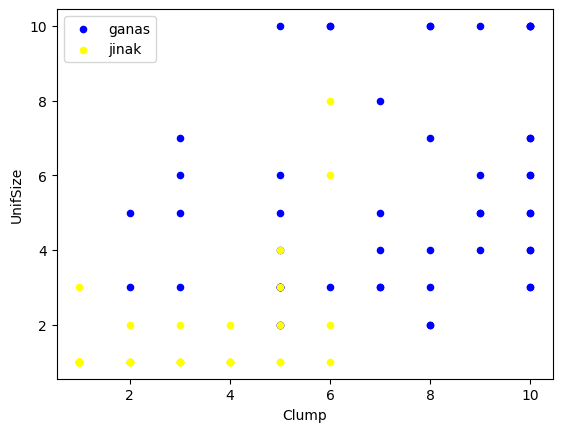

Preprocessing

#cek type dari masing2 feature/kolom
cell_df.dtypes

ID              int64
Clump           int64
UnifSize        int64
UnifShape       int64
MargAdh         int64
SingEpiSize     int64
BareNuc        object
BlandChrom      int64
NormNucl        int64
Mit             int64
Class           int64
dtype: object

cell_df = cell_df[pd.to_numeric(cell_df['BareNuc'],errors="coerce").notnull()] #mengatasi value yg error menjadi NaN
cell_df['BareNuc']=cell_df['BareNuc'].astype('int') #mengubah type menjadi integer
cell_df.dtypes

ID             int64
Clump          int64
UnifSize       int64
UnifShape      int64
MargAdh        int64
SingEpiSize    int64
BareNuc        int32
BlandChrom     int64
NormNucl       int64
Mit            int64
Class          int64
dtype: object

Train Test Split

#set X
feature_df = cell_df[['Clump', 'UnifSize','UnifShape','MargAdh','SingEpiSize','BareNuc','BlandChrom','NormNucl','Mit']].values
X = np.asarray(feature_df)
X[0:5]

array([[ 5,  1,  1,  1,  2,  1,  3,  1,  1],
       [ 5,  4,  4,  5,  7, 10,  3,  2,  1],
       [ 3,  1,  1,  1,  2,  2,  3,  1,  1],
       [ 6,  8,  8,  1,  3,  4,  3,  7,  1],
       [ 4,  1,  1,  3,  2,  1,  3,  1,  1]], dtype=int64)

#set Y
cell_df['Class'] = cell_df['Class'].astype('int')
y=np.asarray(cell_df['Class'])
y[0:5]

array([2, 2, 2, 2, 2])

#train-test split
train_x,test_x,train_y,test_y=train_test_split(X,y, test_size=0.2,random_state=4)
print('Train set:', train_x.shape,train_y.shape)
print('Train set:', test_x.shape,test_y.shape)

Train set: (546, 9) (546,)
Train set: (137, 9) (137,)

Modelling

#membuat model
from sklearn import svm
clf = svm.SVC(kernel='rbf')
clf.fit(train_x,train_y)

SVC()

In a Jupyter environment, please rerun this cell to show the HTML representation or trust the notebook.
On GitHub, the HTML representation is unable to render, please try loading this page with nbviewer.org.

#Prediksi
yhat = clf.predict(test_x)
yhat[0:5]

array([2, 4, 2, 4, 2])

Evaluasi

#jaccard score
from sklearn.metrics import jaccard_score
jaccard_score(test_y,yhat,pos_label=2)

0.9444444444444444

#f1-score
from sklearn.metrics import f1_score
f1_score(test_y,yhat,pos_label=2)

0.9714285714285714

#visualisasi confusion matrix
from sklearn.metrics import classification_report, confusion_matrix
import itertools
def plot_confusion_matrix(cm, classes,
                          normalize=False,
                          title='Confusion matrix',
                          cmap=plt.cm.Blues):
  """
  This function prints and plots the confusion matrix.
  Normalization can be applied by setting `normalize=True`.
  """
  if normalize:
    cm = cm.astype('float') / cm.sum(axis=1)[:, np.newaxis]
    print("Normalized confusion matrix")
  else:
    print('Confusion matrix, without normalization')
 
  print(cm)

  plt.imshow(cm, interpolation='nearest', cmap=cmap)
  plt.title(title)
  plt.colorbar()
  tick_marks = np.arange(len(classes))
  plt.xticks(tick_marks, classes, rotation=45)
  plt.yticks(tick_marks, classes)
  
  fmt = '.2f' if normalize else 'd'
  thresh = cm.max() / 2.
  for i, j in itertools.product(range(cm.shape[0]), range(cm.shape[1])):
    plt.text(j, i, format(cm[i, j], fmt),
             horizontalalignment="center",
             color="white" if cm[i, j] > thresh else "black")
  plt.tight_layout()
  plt.ylabel('True label')
  plt.xlabel('Predicted label')
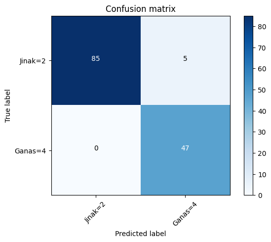
print(confusion_matrix(test_y, yhat, labels=[2,4]))

[[85  5]
 [ 0 47]]

#confusion matrix
cnf_matrix =confusion_matrix(test_y, yhat, labels=[2,4])
plt.figure()
plot_confusion_matrix(cnf_matrix,classes=['Jinak=2', 'Ganas=4'],normalize = False, title='Confusion matrix')

Confusion matrix, without normalization
[[85  5]
 [ 0 47]]