Modul 6 Praktikum Sains Data

Outline

Clustering
K-Means

1. Clustering

Termasuk dalam kategori unsupervised learning (data tidak memiliki label)
Mengelompokkan data data dengan sifat/karakteristik yg sama sebagai satu cluster
Cluster : sekelompok objek yang memiliki kesamaan dengan objek yang ada di cluster tersebut dan berbeda dengan objek di cluster lainnya
Aplikasi : rekomendasi film/musik pada aplikasi, iklan pada sosmed, dll.

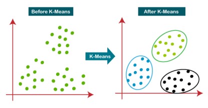
2. K-Means

K-Means bertujuan memperkecil jarak antar data (SSE) dalam cluster dan memperbesar jarak antar cluster

\[SSE = \sum (x_i -c_j)^2\]

Langkah-Langkah: 1. Tentukan centroid untuk k cluster 2. Hitung jarak tiap data dengan centroid 3. Assign data ke centroid terdeka 4. Tentukan centroid baru 5. Ulangi langkah 1 - 4

1. K-means Clustering menggunakan dataset random

Contoh K-Means clustering menggunakan data random.

#import modul yang diperlukan
import random
import numpy as np
import matplotlib.pyplot as plt
from sklearn.cluster import KMeans
from sklearn.datasets import make_blobs
%matplotlib inline

Data

#data
np.random.seed(0)

#membuat sample, dengan centroid sebagai berikut
X, y = make_blobs(n_samples= 5000, centers = [[4,4],[-2,-1],[2,-3],[1,1]], cluster_std=0.9)

#menggambar plot dari sample
plt.scatter(X[:,0], X[:,1],marker='.')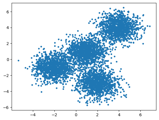

Membuat model

#buat model k-means, jumlah cluster 4, algoritma akan diulang sebanyak 12 kali
k_means = KMeans(init="k-means++", n_clusters = 4, n_init =12)

#fitting x ke model
k_means.fit(X)

KMeans(n_clusters=4, n_init=12)

In a Jupyter environment, please rerun this cell to show the HTML representation or trust the notebook.
On GitHub, the HTML representation is unable to render, please try loading this page with nbviewer.org.

Output hasil clustering

#hasil clustering pada data
k_means_labels = k_means.labels_
k_means_labels

array([0, 3, 3, ..., 1, 0, 0])

#centroid dari 4 cluster setelah menggunakan model k-means
k_means_cluster_centers = k_means.cluster_centers_
k_means_cluster_centers

array([[-2.03743147, -0.99782524],
       [ 3.97334234,  3.98758687],
       [ 0.96900523,  0.98370298],
       [ 1.99741008, -3.01666822]])

#plot hasil clustering
fig = plt.figure(figsize=(6,4))
colors = plt.cm.Spectral(np.linspace(0,1, len(set(k_means_labels))))
ax= fig.add_subplot(1,1,1)
for k, col in zip(range(len([[4,4],[-2,-1],[2,-3],[1,1]])), colors) :
 my_members = (k_means_labels==k)
 cluster_center = k_means_cluster_centers[k]
 ax.plot(X[my_members,0], X[my_members,1], 'w', markerfacecolor=col,marker='.')
 ax.plot(cluster_center[0],cluster_center[1],'o',markerfacecolor=col,markeredgecolor='k',markersize=
6)
ax.set_title('KMeans Clustering')
#hilangkan sumbu
ax.set_xticks(())
ax.set_yticks(())
plt.show()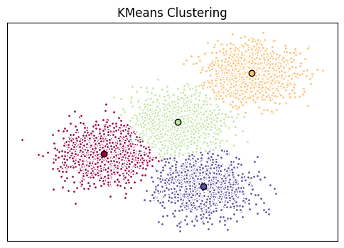

2. Clustering menggunakan dataset (csv)

Pada contoh ini, akan dilakukan clustering menggunakan dataset nasabah bank (Cust_Segmentation.csv). - Kaggle

Nasabah tersebut akan dikelompokkan menjadi 3 cluster.

#import modul dan membaca dataset
import pandas as pd
cust_df = pd.read_csv(r'./Cust_Segmentation.csv')

Data

#cuplikan dataset
cust_df.head()

	Customer Id	Age	Edu	Years Employed	Income	Card Debt	Other Debt	Defaulted	Address	DebtIncomeRatio
0	1	41	2	6	19	0.124	1.073	0.0	NBA001	6.3
1	2	47	1	26	100	4.582	8.218	0.0	NBA021	12.8
2	3	33	2	10	57	6.111	5.802	1.0	NBA013	20.9
3	4	29	2	4	19	0.681	0.516	0.0	NBA009	6.3
4	5	47	1	31	253	9.308	8.908	0.0	NBA008	7.2

#periksa tipe data dari masing masing kolom pada dataset
cust_df.info()

<class 'pandas.core.frame.DataFrame'>
RangeIndex: 850 entries, 0 to 849
Data columns (total 10 columns):
 #   Column           Non-Null Count  Dtype  
---  ------           --------------  -----  
 0   Customer Id      850 non-null    int64  
 1   Age              850 non-null    int64  
 2   Edu              850 non-null    int64  
 3   Years Employed   850 non-null    int64  
 4   Income           850 non-null    int64  
 5   Card Debt        850 non-null    float64
 6   Other Debt       850 non-null    float64
 7   Defaulted        700 non-null    float64
 8   Address          850 non-null    object 
 9   DebtIncomeRatio  850 non-null    float64
dtypes: float64(4), int64(5), object(1)
memory usage: 66.5+ KB

Preprocessing data

#buat semua data menjadi numerik
cust_df2 = cust_df.drop('Address',axis=1)
cust_df2.head()

	Customer Id	Age	Edu	Years Employed	Income	Card Debt	Other Debt	Defaulted	DebtIncomeRatio
0	1	41	2	6	19	0.124	1.073	0.0	6.3
1	2	47	1	26	100	4.582	8.218	0.0	12.8
2	3	33	2	10	57	6.111	5.802	1.0	20.9
3	4	29	2	4	19	0.681	0.516	0.0	6.3
4	5	47	1	31	253	9.308	8.908	0.0	7.2

cust_df2.info()

<class 'pandas.core.frame.DataFrame'>
RangeIndex: 850 entries, 0 to 849
Data columns (total 9 columns):
 #   Column           Non-Null Count  Dtype  
---  ------           --------------  -----  
 0   Customer Id      850 non-null    int64  
 1   Age              850 non-null    int64  
 2   Edu              850 non-null    int64  
 3   Years Employed   850 non-null    int64  
 4   Income           850 non-null    int64  
 5   Card Debt        850 non-null    float64
 6   Other Debt       850 non-null    float64
 7   Defaulted        700 non-null    float64
 8   DebtIncomeRatio  850 non-null    float64
dtypes: float64(4), int64(5)
memory usage: 59.9 KB

#scaling value yang terdapat pada dataset agar error tidak besar
from sklearn.preprocessing import StandardScaler
X = cust_df2.values[:,1:]
X = np.nan_to_num(X)
Clus_dataSet= StandardScaler().fit_transform(X)
Clus_dataSet

array([[ 0.74291541,  0.31212243, -0.37878978, ..., -0.59048916,
        -0.52379654, -0.57652509],
       [ 1.48949049, -0.76634938,  2.5737211 , ...,  1.51296181,
        -0.52379654,  0.39138677],
       [-0.25251804,  0.31212243,  0.2117124 , ...,  0.80170393,
         1.90913822,  1.59755385],
       ...,
       [-1.24795149,  2.46906604, -1.26454304, ...,  0.03863257,
         1.90913822,  3.45892281],
       [-0.37694723, -0.76634938,  0.50696349, ..., -0.70147601,
        -0.52379654, -1.08281745],
       [ 2.1116364 , -0.76634938,  1.09746566, ...,  0.16463355,
        -0.52379654, -0.2340332 ]])

Membuat model

#modelling
clusterNum = 3
k_means_cust = KMeans(init = 'k-means++', n_clusters= clusterNum, n_init = 12) 
#3 cluster, dengan running algoritma sebanyak 12 kali

k_means_cust.fit(X)

#hasil clustering
labels_cust = k_means_cust.labels_
print(labels_cust)

[2 0 2 2 1 0 2 0 2 0 0 2 2 2 2 2 2 2 0 2 2 2 2 0 0 0 2 2 0 2 0 2 2 2 2 2 2
 2 2 0 2 0 2 1 2 0 2 2 2 0 0 2 2 0 0 2 2 2 0 2 0 2 0 0 2 2 0 2 2 2 0 0 0 2
 2 2 2 2 0 2 0 0 1 2 2 2 2 2 2 2 0 2 2 2 2 2 2 2 2 2 2 0 0 2 2 2 2 2 2 0 2
 2 2 2 2 2 2 2 0 2 2 2 2 2 2 0 2 2 2 2 2 0 2 2 2 2 0 2 2 2 2 2 2 2 0 2 0 2
 2 2 2 2 2 2 0 2 0 0 2 0 2 2 0 2 2 2 2 2 2 2 0 2 2 2 2 2 2 2 2 0 2 2 2 0 2
 2 2 2 2 0 2 2 0 2 0 2 2 0 1 2 0 2 2 2 2 2 2 1 0 2 2 2 2 0 2 2 0 0 2 0 2 0
 2 2 2 2 0 2 2 2 2 2 2 2 0 2 2 2 2 2 2 2 2 2 2 1 0 2 2 2 2 2 2 2 0 2 2 2 2
 2 2 0 2 2 0 2 2 0 2 2 2 2 2 2 2 2 2 2 2 2 2 0 0 2 0 2 0 2 0 0 2 2 2 2 2 2
 2 2 2 0 0 0 2 2 2 0 2 2 2 2 2 2 2 2 2 2 2 2 2 2 0 2 0 2 2 2 2 2 0 2 0 0 2
 2 2 2 2 0 2 2 2 2 2 2 0 2 2 0 2 2 0 2 2 2 2 2 0 2 2 2 1 2 2 2 0 2 0 0 0 2
 2 2 0 2 2 2 2 2 2 2 2 2 2 2 0 2 0 2 2 2 2 2 2 2 2 2 2 0 2 2 2 2 2 2 2 2 2
 2 0 2 2 0 2 2 2 2 0 2 2 2 2 0 2 2 0 2 2 2 2 2 2 2 2 2 0 2 2 2 0 2 2 2 2 1
 2 2 2 2 2 2 0 2 2 2 1 2 2 2 2 0 2 1 2 2 2 2 0 2 0 0 0 2 2 0 0 2 2 2 2 2 2
 2 0 2 2 2 2 0 2 2 2 0 2 0 2 2 2 0 2 2 2 2 0 0 2 2 2 2 0 2 2 2 2 0 2 2 2 2
 2 0 0 2 2 2 2 2 2 2 2 2 2 2 1 0 2 2 2 2 2 2 0 2 2 2 2 0 2 2 0 2 2 1 2 1 2
 2 1 2 2 2 2 2 2 2 2 2 0 2 0 2 2 1 2 2 2 2 2 2 2 2 0 2 2 2 2 2 2 2 2 0 2 0
 2 2 2 2 2 2 0 2 2 2 2 0 2 0 2 2 2 2 2 2 2 2 2 2 2 2 2 2 0 2 2 2 2 2 2 2 0
 0 2 2 0 2 0 2 2 0 2 0 2 2 1 2 0 2 0 2 2 2 2 2 0 0 2 2 2 2 0 2 2 2 0 0 2 2
 0 2 2 2 0 2 1 2 2 0 2 2 2 2 2 2 2 0 2 2 2 0 2 2 2 2 2 0 2 2 0 2 2 2 2 2 2
 2 2 0 2 2 0 2 0 2 0 0 2 2 2 0 2 0 2 2 2 2 2 0 2 2 2 2 0 0 2 2 0 0 2 2 2 2
 2 0 2 2 2 2 0 2 2 2 2 2 2 2 2 2 2 2 0 2 0 0 2 0 2 0 0 2 2 0 2 2 2 2 2 0 0
 2 2 2 2 2 2 2 0 2 2 2 2 2 2 1 0 0 2 2 2 2 2 2 2 0 2 2 2 2 2 2 0 2 2 2 2 2
 2 2 2 2 2 2 2 2 2 2 2 0 2 2 2 2 2 2 2 2 2 2 2 2 2 2 2 0 2 2 2 2 2 2 2 0]

#menambahkan kolom hasil clustering pada dataset
cust_df2['Clus_km'] = labels_cust
cust_df2.head(5)

	Customer Id	Age	Edu	Years Employed	Income	Card Debt	Other Debt	Defaulted	DebtIncomeRatio	Clus_km
0	1	41	2	6	19	0.124	1.073	0.0	6.3	2
1	2	47	1	26	100	4.582	8.218	0.0	12.8	0
2	3	33	2	10	57	6.111	5.802	1.0	20.9	2
3	4	29	2	4	19	0.681	0.516	0.0	6.3	2
4	5	47	1	31	253	9.308	8.908	0.0	7.2	1

#melihat rata rata per cluster
cust_df2.groupby('Clus_km').mean()

	Customer Id	Age	Edu	Years Employed	Income	Card Debt	Other Debt	Defaulted	DebtIncomeRatio
Clus_km
0	402.295082	41.333333	1.956284	15.256831	83.928962	3.103639	5.765279	0.171233	10.724590
1	410.166667	45.388889	2.666667	19.555556	227.166667	5.678444	10.907167	0.285714	7.322222
2	432.468413	32.964561	1.614792	6.374422	31.164869	1.032541	2.104133	0.285185	10.094761

#plot hasil clustering berdasarkan age dan income
area = np.pi * (X[:, 1])**2
plt.scatter(X[:,0],X[:,3],s = area, c = labels_cust.astype(float), alpha=0.5)
plt.xlabel('Age',fontsize=18)
plt.ylabel('Income',fontsize = 16)
plt.show()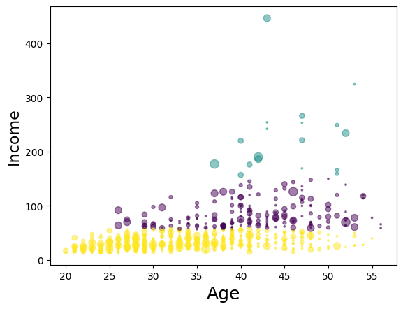

Kesimpulan

Dari datset diatas, kita dapat membuat 3 cluster, dengan segmentasi sebagai berikut:

Kuning : dewasa muda, pendapatan rendah
Ungu: dewasa menengah, pendapatan kelas menengah
Hijau: dewasa tua, pendapatan tinggi