Pertemuan 3 : Simple Data Visualization (matplotlib)

Data visualization in python using matplotlib (pyplot)
Published

April 23, 2024

Kembali ke EDA

Matplotlib (Pyplot)

Matplotlib adalah library yang digunakan untuk visualisasi data. Hasil visualisasi data matplotllib menyerupai hasil visualisasi pada bahasa pemrograman matlab. Library ini bukanlah cara yang paling mudah untuk menghasilkan visualisasi data, tetapi visualisasi yang dihasilkan fleksibel dan dapat digunakan untuk banyak sekali kasus.


Download dataset

import numpy as np
import pandas as pd
import matplotlib.pyplot as plt

# Import Dataset
df = pd.read_csv('https://raw.githubusercontent.com/farhanage/dataset-for-study/main/insurance.csv')

# Cek 5 observasi pertama
df.head()
age sex bmi children smoker region charges
0 19 female 27.900 0 yes southwest 16884.92400
1 18 male 33.770 1 no southeast 1725.55230
2 28 male 33.000 3 no southeast 4449.46200
3 33 male 22.705 0 no northwest 21984.47061
4 32 male 28.880 0 no northwest 3866.85520
# melihat informasi mengenai tiap variabel
df.info()
<class 'pandas.core.frame.DataFrame'>
RangeIndex: 1338 entries, 0 to 1337
Data columns (total 7 columns):
 #   Column    Non-Null Count  Dtype  
---  ------    --------------  -----  
 0   age       1338 non-null   int64  
 1   sex       1338 non-null   object 
 2   bmi       1338 non-null   float64
 3   children  1338 non-null   int64  
 4   smoker    1338 non-null   object 
 5   region    1338 non-null   object 
 6   charges   1338 non-null   float64
dtypes: float64(2), int64(2), object(3)
memory usage: 73.3+ KB
# statistik deskritif semua variabel numerik
df.describe()
age bmi children charges
count 1338.000000 1338.000000 1338.000000 1338.000000
mean 39.207025 30.663397 1.094918 13270.422265
std 14.049960 6.098187 1.205493 12110.011237
min 18.000000 15.960000 0.000000 1121.873900
25% 27.000000 26.296250 0.000000 4740.287150
50% 39.000000 30.400000 1.000000 9382.033000
75% 51.000000 34.693750 2.000000 16639.912515
max 64.000000 53.130000 5.000000 63770.428010

Box Plot

# Box Plot variabel `age`
plt.boxplot(x='age', data=df)

# Menambahkan Judul Plot
plt.title("Box Plot")
 
# Menambahkan label sumbu X dan Y
plt.xlabel('Age')
plt.ylabel('Value')

# Menunjukkan plot
plt.show()

# Box Plot variabel `bmi`
plt.boxplot(x='bmi', data=df)

# Menambahkan Judul Plot
plt.title("Box Plot")
 
# Menambahkan label sumbu X dan Y
plt.xlabel('bmi')
plt.ylabel('Value')

# Menunjukkan plot
plt.show()

Note

Seperti halnya penggunaan syntax ? pada bahasa pemrograman R, kita dapat mengakses dokumentasi suatu fungsi dalam suatu modul pada python dengan menggunakan function help()

# Melihat dokumentasi mengenai function plt.boxplot()
help(plt.boxplot)
Help on function boxplot in module matplotlib.pyplot:

boxplot(x: 'ArrayLike | Sequence[ArrayLike]', notch: 'bool | None' = None, sym: 'str | None' = None, vert: 'bool | None' = None, whis: 'float | tuple[float, float] | None' = None, positions: 'ArrayLike | None' = None, widths: 'float | ArrayLike | None' = None, patch_artist: 'bool | None' = None, bootstrap: 'int | None' = None, usermedians: 'ArrayLike | None' = None, conf_intervals: 'ArrayLike | None' = None, meanline: 'bool | None' = None, showmeans: 'bool | None' = None, showcaps: 'bool | None' = None, showbox: 'bool | None' = None, showfliers: 'bool | None' = None, boxprops: 'dict[str, Any] | None' = None, labels: 'Sequence[str] | None' = None, flierprops: 'dict[str, Any] | None' = None, medianprops: 'dict[str, Any] | None' = None, meanprops: 'dict[str, Any] | None' = None, capprops: 'dict[str, Any] | None' = None, whiskerprops: 'dict[str, Any] | None' = None, manage_ticks: 'bool' = True, autorange: 'bool' = False, zorder: 'float | None' = None, capwidths: 'float | ArrayLike | None' = None, *, data=None) -> 'dict[str, Any]'
    Draw a box and whisker plot.

    The box extends from the first quartile (Q1) to the third
    quartile (Q3) of the data, with a line at the median.
    The whiskers extend from the box to the farthest data point
    lying within 1.5x the inter-quartile range (IQR) from the box.
    Flier points are those past the end of the whiskers.
    See https://en.wikipedia.org/wiki/Box_plot for reference.

    .. code-block:: none

              Q1-1.5IQR   Q1   median  Q3   Q3+1.5IQR
                           |-----:-----|
           o      |--------|     :     |--------|    o  o
                           |-----:-----|
         flier             <----------->            fliers
                                IQR


    Parameters
    ----------
    x : Array or a sequence of vectors.
        The input data.  If a 2D array, a boxplot is drawn for each column
        in *x*.  If a sequence of 1D arrays, a boxplot is drawn for each
        array in *x*.

    notch : bool, default: False
        Whether to draw a notched boxplot (`True`), or a rectangular
        boxplot (`False`).  The notches represent the confidence interval
        (CI) around the median.  The documentation for *bootstrap*
        describes how the locations of the notches are computed by
        default, but their locations may also be overridden by setting the
        *conf_intervals* parameter.

        .. note::

            In cases where the values of the CI are less than the
            lower quartile or greater than the upper quartile, the
            notches will extend beyond the box, giving it a
            distinctive "flipped" appearance. This is expected
            behavior and consistent with other statistical
            visualization packages.

    sym : str, optional
        The default symbol for flier points.  An empty string ('') hides
        the fliers.  If `None`, then the fliers default to 'b+'.  More
        control is provided by the *flierprops* parameter.

    vert : bool, default: True
        If `True`, draws vertical boxes.
        If `False`, draw horizontal boxes.

    whis : float or (float, float), default: 1.5
        The position of the whiskers.

        If a float, the lower whisker is at the lowest datum above
        ``Q1 - whis*(Q3-Q1)``, and the upper whisker at the highest datum
        below ``Q3 + whis*(Q3-Q1)``, where Q1 and Q3 are the first and
        third quartiles.  The default value of ``whis = 1.5`` corresponds
        to Tukey's original definition of boxplots.

        If a pair of floats, they indicate the percentiles at which to
        draw the whiskers (e.g., (5, 95)).  In particular, setting this to
        (0, 100) results in whiskers covering the whole range of the data.

        In the edge case where ``Q1 == Q3``, *whis* is automatically set
        to (0, 100) (cover the whole range of the data) if *autorange* is
        True.

        Beyond the whiskers, data are considered outliers and are plotted
        as individual points.

    bootstrap : int, optional
        Specifies whether to bootstrap the confidence intervals
        around the median for notched boxplots. If *bootstrap* is
        None, no bootstrapping is performed, and notches are
        calculated using a Gaussian-based asymptotic approximation
        (see McGill, R., Tukey, J.W., and Larsen, W.A., 1978, and
        Kendall and Stuart, 1967). Otherwise, bootstrap specifies
        the number of times to bootstrap the median to determine its
        95% confidence intervals. Values between 1000 and 10000 are
        recommended.

    usermedians : 1D array-like, optional
        A 1D array-like of length ``len(x)``.  Each entry that is not
        `None` forces the value of the median for the corresponding
        dataset.  For entries that are `None`, the medians are computed
        by Matplotlib as normal.

    conf_intervals : array-like, optional
        A 2D array-like of shape ``(len(x), 2)``.  Each entry that is not
        None forces the location of the corresponding notch (which is
        only drawn if *notch* is `True`).  For entries that are `None`,
        the notches are computed by the method specified by the other
        parameters (e.g., *bootstrap*).

    positions : array-like, optional
        The positions of the boxes. The ticks and limits are
        automatically set to match the positions. Defaults to
        ``range(1, N+1)`` where N is the number of boxes to be drawn.

    widths : float or array-like
        The widths of the boxes.  The default is 0.5, or ``0.15*(distance
        between extreme positions)``, if that is smaller.

    patch_artist : bool, default: False
        If `False` produces boxes with the Line2D artist. Otherwise,
        boxes are drawn with Patch artists.

    labels : sequence, optional
        Labels for each dataset (one per dataset).

    manage_ticks : bool, default: True
        If True, the tick locations and labels will be adjusted to match
        the boxplot positions.

    autorange : bool, default: False
        When `True` and the data are distributed such that the 25th and
        75th percentiles are equal, *whis* is set to (0, 100) such
        that the whisker ends are at the minimum and maximum of the data.

    meanline : bool, default: False
        If `True` (and *showmeans* is `True`), will try to render the
        mean as a line spanning the full width of the box according to
        *meanprops* (see below).  Not recommended if *shownotches* is also
        True.  Otherwise, means will be shown as points.

    zorder : float, default: ``Line2D.zorder = 2``
        The zorder of the boxplot.

    Returns
    -------
    dict
      A dictionary mapping each component of the boxplot to a list
      of the `.Line2D` instances created. That dictionary has the
      following keys (assuming vertical boxplots):

      - ``boxes``: the main body of the boxplot showing the
        quartiles and the median's confidence intervals if
        enabled.

      - ``medians``: horizontal lines at the median of each box.

      - ``whiskers``: the vertical lines extending to the most
        extreme, non-outlier data points.

      - ``caps``: the horizontal lines at the ends of the
        whiskers.

      - ``fliers``: points representing data that extend beyond
        the whiskers (fliers).

      - ``means``: points or lines representing the means.

    Other Parameters
    ----------------
    showcaps : bool, default: True
        Show the caps on the ends of whiskers.
    showbox : bool, default: True
        Show the central box.
    showfliers : bool, default: True
        Show the outliers beyond the caps.
    showmeans : bool, default: False
        Show the arithmetic means.
    capprops : dict, default: None
        The style of the caps.
    capwidths : float or array, default: None
        The widths of the caps.
    boxprops : dict, default: None
        The style of the box.
    whiskerprops : dict, default: None
        The style of the whiskers.
    flierprops : dict, default: None
        The style of the fliers.
    medianprops : dict, default: None
        The style of the median.
    meanprops : dict, default: None
        The style of the mean.
    data : indexable object, optional
        If given, all parameters also accept a string ``s``, which is
        interpreted as ``data[s]`` (unless this raises an exception).

    See Also
    --------
    violinplot : Draw an estimate of the probability density function.

Histogram

# Histogram variabel `bmi`
plt.hist(x='bmi', data=df)

# Menambahkan Judul Plot
plt.title("Histogram")
 
# Menambahkan label sumbu X dan Y
plt.xlabel('bmi')
plt.ylabel('Count')

# Menunjukkan plot
plt.show()

Bar Chart

# Hitung banyaknya responden dari masing-masing gender
df['sex'].value_counts()
sex
male      676
female    662
Name: count, dtype: int64
# Bar chart jumlah tiap jenis kelamin
df['sex'].value_counts().plot(kind='bar')

# Menambahkan Judul Plot
plt.title("Bar Chart")
 
# Menambahkan label sumbu X dan Y
plt.xlabel('sex')
plt.ylabel('count')

# Menunjukkan plot
plt.show()

Horizontal Bar Chart

# Horizontal Bar chart jumlah tiap jenis kelamin
df['sex'].value_counts().plot(kind='barh')

# Menambahkan Judul Plot
plt.title("Bar Chart")
 
# Menambahkan label sumbu X dan Y
plt.xlabel('count')
plt.ylabel('sex')

# Menunjukkan plot
plt.show()

Pie Chart

# Pie chart persentase sebaran region seluruh responden
df['region'].value_counts().plot(kind='pie', autopct='%1.1f%%')

# Menambahkan Judul Plot
plt.title("Pie Chart")

# Menunjukkan plot
plt.show()

Scatter Plot

# Scatter plot variabel `age` dan `charges`
df.plot(kind='scatter', x='age', y='charges')

# Menambahkan Judul Plot
plt.title("Scatter Plot `Age` vs `Charges`")
 
# Menambahkan label sumbu X dan Y
plt.xlabel('Age')
plt.ylabel('Charges')

# Menunjukkan plot
plt.show()


Untuk plot lainnya, silakan telusuri dokumentasi dari library matplotlib yang dapat diakses pada link berikut : Dokumentasi matplotlib.pyplot

Subplots

Figure and Axes

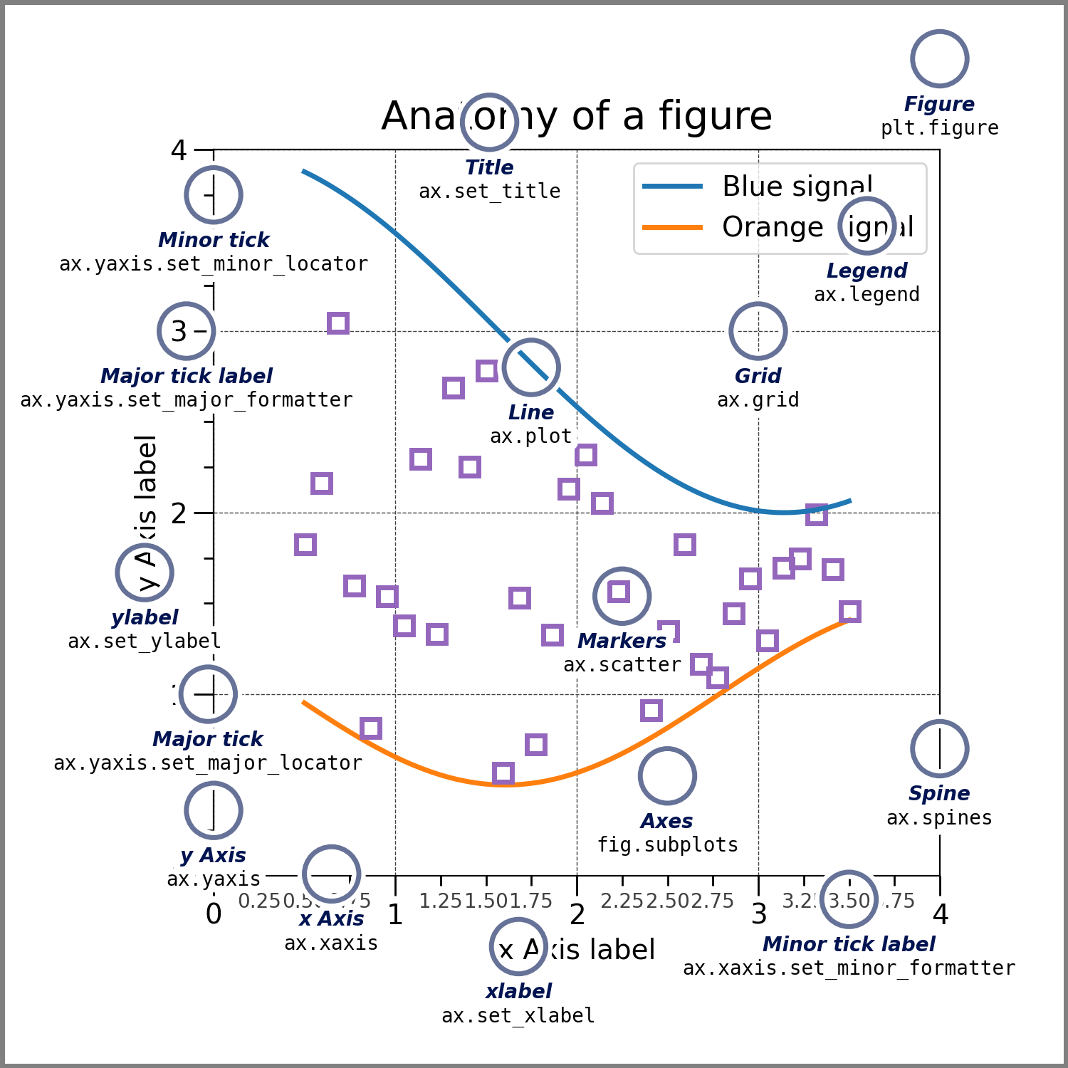
Pembuatan suatu plot menggunakan library matplotlib akan menghasilkan suatu figure yang memiliki beberapa komponen di dalamnya.

Berikut cara membuat suatu figure menggunakan matplotlib

fig = plt.figure()  # an empty figure with no Axes

plt.show()
<Figure size 672x480 with 0 Axes>

Figure kosong tidak dapat divisualisasikan. Untuk membuat suatu figure yang memiliki axes, gunakan function plt.subplots()

fig, ax = plt.subplots()  # a figure with a single Axes

plt.show()

Bagaimana jika kita ingin membuat gabungan dari beberapa Axes dalam 1 figure?

function subplots menerima parameter jumlah baris dan jumlah kolom untuk membentuk suatu grid yang terdiri atas 1 atau lebih axes

fig, axs = plt.subplots(2, 2)  # a figure with a 2x2 grid of Axes

plt.show()

Selain dengan function subplots, ada juga function subplot_mosaic yang akan menghasilkan axes dengan ukuran yang lebih bervariasi.

# a figure with one axes on the left, and two on the right:
fig, axs = plt.subplot_mosaic([['left', 'right_top'],
                               ['left', 'right_bottom']])

plt.show()

Plots

Untuk menambahkan plot pada tiap axis, gunakan function-function plot pada axis dengan index yang bersesuaian.

fig, axs = plt.subplots(2, 2, layout="constrained")

axs[0,0].hist(df['age'])

axs[0,0].set_title('Variabel `Age`')

axs[0,1].hist(df['bmi'])

axs[0,1].set_title('Variabel `bmi`')

axs[1,0].hist(df['children'])

axs[1,0].set_title('Variabel `children`')

axs[1,1].hist(df['charges'])

axs[1,1].set_title('Variabel `charges`')

fig.suptitle('Histogram Variabel Numerik')

plt.show()

Lebih lanjut, silakan baca dokumentasi dari plt.subplot pada link berikut : Dokumentasi plt.subplots