#import modul
import numpy as np
import matplotlib.pyplot as plt
import pandas as pd
%matplotlib inlineModul 6 Praktikum Sains Data: K-Nearest Neighbor, K-Means Clustering
Kembali ke Sains Data
K-Nearest Neighbor
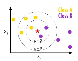
K-Nearest neighbor adalah salah satu jenis algoritma supervised learning. Biasanya, algoritma ini digunakan untuk masalah klasifikasi. Kelas dari data tersebut ditentukan dari sejumlah k titik yang berperan “tetangga”. Pada gambar di atas, ketika k = 3, bintang akan diklasifikasikan sebagai kelas ungu, sebab mayoritas dari tetangganya adalah ungu. Sedangkan, ketika k = 6, bintang akan diklasifikasikan sebagai kelas kuning.
Data
Pada module kali ini, akan digunakan data csv teleCust1000t (teleCust1000t.csv) yang bisa didownload dari:
- Direct link (langsung dari GitHub Pages ini)
- Kaggle: https://www.kaggle.com/code/zohaib123/telecusts-prediction-k-nearest-neighbors
 #membaca dataset
df = pd.read_csv('./teleCust1000t.csv')
df.head()| region | tenure | age | marital | address | income | ed | employ | retire | gender | reside | custcat | |
|---|---|---|---|---|---|---|---|---|---|---|---|---|
| 0 | 2 | 13 | 44 | 1 | 9 | 64.0 | 4 | 5 | 0.0 | 0 | 2 | 1 |
| 1 | 3 | 11 | 33 | 1 | 7 | 136.0 | 5 | 5 | 0.0 | 0 | 6 | 4 |
| 2 | 3 | 68 | 52 | 1 | 24 | 116.0 | 1 | 29 | 0.0 | 1 | 2 | 3 |
| 3 | 2 | 33 | 33 | 0 | 12 | 33.0 | 2 | 0 | 0.0 | 1 | 1 | 1 |
| 4 | 2 | 23 | 30 | 1 | 9 | 30.0 | 1 | 2 | 0.0 | 0 | 4 | 3 |
#menghitung jumlah anggota tiap kelas
df['custcat'].value_counts()
custcat
3 281
1 266
4 236
2 217
Name: count, dtype: int64 #melihat sebaran income dengan histogram
df.hist(column='income')array([[<Axes: title={'center': 'income'}>]], dtype=object)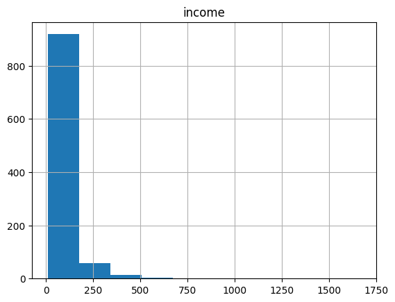
#melihat 4 row pertama
X = df.drop(columns="custcat")
X.head(4)| region | tenure | age | marital | address | income | ed | employ | retire | gender | reside | |
|---|---|---|---|---|---|---|---|---|---|---|---|
| 0 | 2 | 13 | 44 | 1 | 9 | 64.0 | 4 | 5 | 0.0 | 0 | 2 |
| 1 | 3 | 11 | 33 | 1 | 7 | 136.0 | 5 | 5 | 0.0 | 0 | 6 |
| 2 | 3 | 68 | 52 | 1 | 24 | 116.0 | 1 | 29 | 0.0 | 1 | 2 |
| 3 | 2 | 33 | 33 | 0 | 12 | 33.0 | 2 | 0 | 0.0 | 1 | 1 |
#melihat kelas dari 4 row pertama
y = df['custcat']
y.head(4)
0 1
1 4
2 3
3 1
Name: custcat, dtype: int64Preprocessing: normalisasi
Normalisasi adalah melakukan scaling pada keseluruhan data sehingga berada dalam rentang interval \([0, 1]\). Normalisasi bisa meningkatkan akurasi KNN karena
- data semua fitur berada di rentang yang sama, sehingga tidak ada bias (bias dalam artian lebih memperhatikan fitur lain karena rentangnya lebih besar sehingga perhitungan jarak menjadi lebih dipengaruhi oleh fitur lain itu)
- bilangan floating-point paling presisi di interval \([0, 1]\)
sklearn menyediakan class untuk normalisasi bernama MinMaxScaler. Sebenarnya min-max scaler ini bisa diubah intervalnya selain \([0,1]\), dengan mengubah parameter feature_range=(0, 1) tetapi tidak kita lakukan
from sklearn.preprocessing import MinMaxScaler#normalize data
X_minmax = MinMaxScaler(feature_range=(0, 1))
X_minmax.fit(X)
X_sc = X_minmax.transform(X.astype(float))X_sc[0:4]array([[0.5 , 0.16901408, 0.44067797, 1. , 0.16363636,
0.0331525 , 0.75 , 0.10638298, 0. , 0. ,
0.14285714],
[1. , 0.14084507, 0.25423729, 1. , 0.12727273,
0.07655214, 1. , 0.10638298, 0. , 0. ,
0.71428571],
[1. , 0.94366197, 0.57627119, 1. , 0.43636364,
0.06449668, 0. , 0.61702128, 0. , 1. ,
0.14285714],
[0.5 , 0.45070423, 0.25423729, 0. , 0.21818182,
0.01446655, 0.25 , 0. , 0. , 1. ,
0. ]])Train test split
from sklearn.model_selection import train_test_split#train test split
X_train, X_test, y_train, y_test = train_test_split(X, y, test_size = 0.2, random_state = 42)print(X_train.shape)
print(y_train.shape)
print(X_test.shape)
print(y_test.shape)(800, 11)
(800,)
(200, 11)
(200,)Membuat model
from sklearn.neighbors import KNeighborsClassifier#membuat model dengan k = 4
k = 4
tele_KNN = KNeighborsClassifier(n_neighbors = k)
tele_KNN.fit(X_train, y_train)KNeighborsClassifier(n_neighbors=4)In a Jupyter environment, please rerun this cell to show the HTML representation or trust the notebook.
On GitHub, the HTML representation is unable to render, please try loading this page with nbviewer.org.
KNeighborsClassifier(n_neighbors=4)
Prediksi
#hasil prediksi
y_pred = tele_KNN.predict(X_test)
y_pred[0:5]
array([3, 2, 1, 3, 1])#kelas sebenarnya
y_test[0:5]521 2
737 1
740 2
660 3
411 1
Name: custcat, dtype: int64Evaluasi Model
from sklearn import metrics#menghitung akurasi
metrics.accuracy_score(y_test, y_pred)0.3Membuat model dengan k lainnya
#membuat model dengan k = 6
k = 6
tele_KNN_6 = KNeighborsClassifier(n_neighbors = k).fit(X_train, y_train)
#hasil prediksi
y_pred_6 = tele_KNN_6.predict(X_test)
y_pred_6[0:5]array([3, 2, 1, 3, 1])#kelas sebenarnya
y_test[0:5]521 2
737 1
740 2
660 3
411 1
Name: custcat, dtype: int64#akurasi
metrics.accuracy_score(y_test, y_pred_6)0.33Hyperparameter Tuning: mencari k terbaik
Kinerja model K-NN sangat bergantung pada jumlah k yang dipilih. Kita bisa saja menentukan k terbaik secara manual menggunakan loop.
#mencari k terbaik diantara 1<=k<=10
nk = 10

mean_acc= np.zeros((nk))
std_acc = np.zeros((nk))

for n in range(1,nk+1):
 neighbor_k = KNeighborsClassifier(n_neighbors= n).fit(X_train,Y_train)
 ypredict = neighbor_k.predict(X_test)
 mean_acc[n-1] = metrics.accuracy_score(Y_test, ypredict)
 std_acc[n-1]= np.std(ypredict==Y_test)/np.sqrt(ypredict.shape[0])

mean_acc
c:\Users\ACER\AppData\Local\Programs\Python\Python312\Lib\site-packages\sklearn\neighbors\_classification.py:238: DataConversionWarning: A column-vector y was passed when a 1d array was expected. Please change the shape of y to (n_samples,), for example using ravel().
return self._fit(X, y)
c:\Users\ACER\AppData\Local\Programs\Python\Python312\Lib\site-packages\sklearn\neighbors\_classification.py:238: DataConversionWarning: A column-vector y was passed when a 1d array was expected. Please change the shape of y to (n_samples,), for example using ravel().
return self._fit(X, y)
c:\Users\ACER\AppData\Local\Programs\Python\Python312\Lib\site-packages\sklearn\neighbors\_classification.py:238: DataConversionWarning: A column-vector y was passed when a 1d array was expected. Please change the shape of y to (n_samples,), for example using ravel().
return self._fit(X, y)
c:\Users\ACER\AppData\Local\Programs\Python\Python312\Lib\site-packages\sklearn\neighbors\_classification.py:238: DataConversionWarning: A column-vector y was passed when a 1d array was expected. Please change the shape of y to (n_samples,), for example using ravel().
return self._fit(X, y)
c:\Users\ACER\AppData\Local\Programs\Python\Python312\Lib\site-packages\sklearn\neighbors\_classification.py:238: DataConversionWarning: A column-vector y was passed when a 1d array was expected. Please change the shape of y to (n_samples,), for example using ravel().
return self._fit(X, y)
c:\Users\ACER\AppData\Local\Programs\Python\Python312\Lib\site-packages\sklearn\neighbors\_classification.py:238: DataConversionWarning: A column-vector y was passed when a 1d array was expected. Please change the shape of y to (n_samples,), for example using ravel().
return self._fit(X, y)
c:\Users\ACER\AppData\Local\Programs\Python\Python312\Lib\site-packages\sklearn\neighbors\_classification.py:238: DataConversionWarning: A column-vector y was passed when a 1d array was expected. Please change the shape of y to (n_samples,), for example using ravel().
return self._fit(X, y)
c:\Users\ACER\AppData\Local\Programs\Python\Python312\Lib\site-packages\sklearn\neighbors\_classification.py:238: DataConversionWarning: A column-vector y was passed when a 1d array was expected. Please change the shape of y to (n_samples,), for example using ravel().
return self._fit(X, y)
c:\Users\ACER\AppData\Local\Programs\Python\Python312\Lib\site-packages\sklearn\neighbors\_classification.py:238: DataConversionWarning: A column-vector y was passed when a 1d array was expected. Please change the shape of y to (n_samples,), for example using ravel().
return self._fit(X, y)
c:\Users\ACER\AppData\Local\Programs\Python\Python312\Lib\site-packages\sklearn\neighbors\_classification.py:238: DataConversionWarning: A column-vector y was passed when a 1d array was expected. Please change the shape of y to (n_samples,), for example using ravel().
return self._fit(X, y)array([0.3 , 0.29 , 0.315, 0.32 , 0.315, 0.31 , 0.335, 0.325, 0.34 ,
0.33 ])#plot akurasi dari beberapa k
plt.plot(range(1,nk+1),mean_acc,'g')
plt.fill_between(range(1,nk+1),mean_acc-1*std_acc,mean_acc+1*std_acc,alpha = 0.10)
plt.fill_between(range(1,nk+1),mean_acc-3*std_acc,mean_acc+3*std_acc,alpha = 0.10, color = "red")
plt.legend(('Accuracy', '+-1xstd', '+-3xstd'))
plt.ylabel('Accuracy')
plt.xlabel('Jumlah neighbor')
plt.tight_layout()
plt.show()
#plot akurasi dari beberapa k
plt.plot(range(1,nk+1),mean_acc,'g')
plt.fill_between(range(1,nk+1),mean_acc-1*std_acc,mean_acc+1*std_acc,alpha = 0.10)
plt.fill_between(range(1,nk+1),mean_acc-3*std_acc,mean_acc+3*std_acc,alpha = 0.10, color = "red")
plt.legend(('Accuracy', '+-1xstd', '+-3xstd'))
plt.ylabel('Accuracy')
plt.xlabel('Jumlah neighbor')
plt.tight_layout()
plt.show()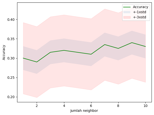
#k terbaik beserta hasilnya
print("akurasi terbaik model adalah", mean_acc.max(), "dengan jumlah k=", mean_acc.argmax()+1)
akurasi terbaik model adalah 0.34 dengan jumlah k= 9Daripada cara manual, kita bisa menggunakan fitur grid search dari scikit-learn.
from sklearn.model_selection import GridSearchCVBuatlah dictionary berisi semua nilai yang ingin dicoba untuk tiap parameter:
KNN_param_grid = {
    'n_neighbors': [1, 2, 3, 4, 5, 6, 7, 8, 9, 10]
}
KNN_auto = KNeighborsClassifier()
KNN_grid_search = GridSearchCV(KNN_auto, KNN_param_grid, scoring="accuracy")# Lakukan grid search
KNN_grid_search.fit(X_train, y_train)GridSearchCV(cv=5, estimator=KNeighborsClassifier(),
param_grid={'n_neighbors': [1, 2, 3, 4, 5, 6, 7, 8, 9, 10]},
scoring='accuracy')In a Jupyter environment, please rerun this cell to show the HTML representation or trust the notebook. On GitHub, the HTML representation is unable to render, please try loading this page with nbviewer.org.
GridSearchCV(cv=5, estimator=KNeighborsClassifier(),
             param_grid={'n_neighbors': [1, 2, 3, 4, 5, 6, 7, 8, 9, 10]},
scoring='accuracy')KNeighborsClassifier()
KNeighborsClassifier()
Lihat hasilnya:
print(KNN_grid_search.best_params_){'n_neighbors': 9}print(KNN_grid_search.best_score_)0.34500000000000003Sehingga nilai k terbaik (dari 1 sampai 10) adalah 9 dengan akurasi 0.345
Clustering
- Termasuk dalam kategori unsupervised learning (data tidak memiliki label)
- Mengelompokkan data data dengan sifat/karakteristik yg sama sebagai satu cluster
- Cluster : sekelompok objek yang memiliki kesamaan dengan objek yang ada di cluster tersebut dan berbeda dengan objek di cluster lainnya
- Aplikasi : rekomendasi film/musik pada aplikasi, iklan pada sosmed, dll.
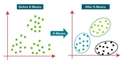
K-Means Clustering
K-Means bertujuan memperkecil jarak antar data (SSE) dalam cluster dan memperbesar jarak antar cluster
\[SSE = \sum (x_i -c_j)^2\]
Langkah-Langkah: 1. Tentukan centroid untuk k cluster 2. Hitung jarak tiap data dengan centroid 3. Assign data ke centroid terdeka 4. Tentukan centroid baru 5. Ulangi langkah 1 - 4
K-means Clustering menggunakan dataset random
Contoh K-Means clustering menggunakan data random.
#import modul yang diperlukan
import numpy as np
import matplotlib.pyplot as plt
from sklearn.cluster import KMeans
from sklearn.datasets import make_blobs
%matplotlib inline
Data
#data
np.random.seed(0)
#membuat sample, dengan centroid sebagai berikut
X, y = make_blobs(n_samples= 5000, centers = [[4,4],[-2,-1],[2,-3],[1,1]], cluster_std=0.9)#menggambar plot dari sample
plt.scatter(X[:,0], X[:,1],marker='.')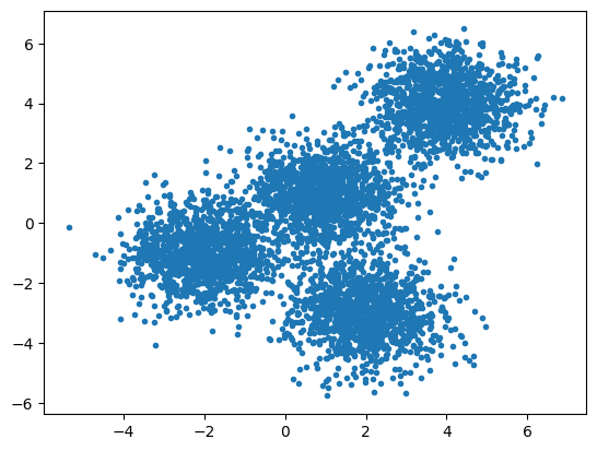
Membuat model
#buat model k-means, jumlah cluster 4, algoritma akan diulang sebanyak 12 kali
k_means = KMeans(init="k-means++", n_clusters = 4, n_init = 12)
#fitting x ke model
k_means.fit(X)KMeans(n_clusters=4, n_init=12)In a Jupyter environment, please rerun this cell to show the HTML representation or trust the notebook.
On GitHub, the HTML representation is unable to render, please try loading this page with nbviewer.org.
KMeans(n_clusters=4, n_init=12)
Output hasil clustering
#hasil clustering pada data
k_means_labels = k_means.labels_
k_means_labels
array([0, 3, 3, ..., 1, 0, 0], dtype=int32)#centroid dari 4 cluster setelah menggunakan model k-means
k_means_cluster_centers = k_means.cluster_centers_
k_means_cluster_centersarray([[-2.03743147, -0.99782524],
[ 3.97334234, 3.98758687],
[ 0.96900523, 0.98370298],
[ 1.99741008, -3.01666822]])#plot hasil clustering
fig = plt.figure(figsize=(6,4))
colors = plt.cm.Spectral(np.linspace(0,1, len(set(k_means_labels))))
ax= fig.add_subplot(1,1,1)
for k, col in zip(range(len([[4,4],[-2,-1],[2,-3],[1,1]])), colors) :
my_members = (k_means_labels==k)
cluster_center = k_means_cluster_centers[k]
ax.plot(X[my_members,0], X[my_members,1], 'w', markerfacecolor=col,marker='.')
ax.plot(cluster_center[0],cluster_center[1],'o',markerfacecolor=col,markeredgecolor='k',markersize=
6)
ax.set_title('KMeans Clustering')
#hilangkan sumbu
ax.set_xticks(())
ax.set_yticks(())
plt.show()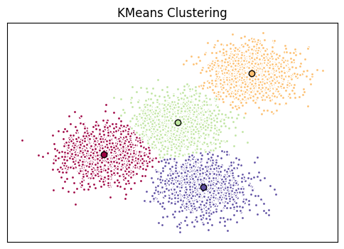
K-Means Clustering menggunakan dataset (csv)
Pada contoh ini, akan dilakukan clustering menggunakan dataset nasabah bank (Cust_Segmentation.csv).
- Direct link (langsung dari GitHub Pages ini)
- Kaggle: https://www.kaggle.com/datasets/sam1o1/cust-segmentation
Nasabah tersebut akan dikelompokkan menjadi 3 cluster.
#import modul dan membaca dataset
import pandas as pd
cust_df = pd.read_csv('./Cust_Segmentation.csv')
Data
#cuplikan dataset
cust_df.head()| Customer Id | Age | Edu | Years Employed | Income | Card Debt | Other Debt | Defaulted | Address | DebtIncomeRatio | |
|---|---|---|---|---|---|---|---|---|---|---|
| 0 | 1 | 41 | 2 | 6 | 19 | 0.124 | 1.073 | 0.0 | NBA001 | 6.3 |
| 1 | 2 | 47 | 1 | 26 | 100 | 4.582 | 8.218 | 0.0 | NBA021 | 12.8 |
| 2 | 3 | 33 | 2 | 10 | 57 | 6.111 | 5.802 | 1.0 | NBA013 | 20.9 |
| 3 | 4 | 29 | 2 | 4 | 19 | 0.681 | 0.516 | 0.0 | NBA009 | 6.3 |
| 4 | 5 | 47 | 1 | 31 | 253 | 9.308 | 8.908 | 0.0 | NBA008 | 7.2 |
#periksa tipe data dari masing masing kolom pada dataset
cust_df.info()
<class 'pandas.core.frame.DataFrame'>
RangeIndex: 850 entries, 0 to 849
Data columns (total 10 columns):
# Column Non-Null Count Dtype
--- ------ -------------- -----
0 Customer Id 850 non-null int64
1 Age 850 non-null int64
2 Edu 850 non-null int64
3 Years Employed 850 non-null int64
4 Income 850 non-null int64
5 Card Debt 850 non-null float64
6 Other Debt 850 non-null float64
7 Defaulted 700 non-null float64
8 Address 850 non-null object
9 DebtIncomeRatio 850 non-null float64
dtypes: float64(4), int64(5), object(1)
memory usage: 66.5+ KBPreprocessing, dan standarisasi
#buat semua data menjadi numerik
cust_df2 = cust_df.drop('Address',axis=1)
cust_df2.head()| Customer Id | Age | Edu | Years Employed | Income | Card Debt | Other Debt | Defaulted | DebtIncomeRatio | |
|---|---|---|---|---|---|---|---|---|---|
| 0 | 1 | 41 | 2 | 6 | 19 | 0.124 | 1.073 | 0.0 | 6.3 |
| 1 | 2 | 47 | 1 | 26 | 100 | 4.582 | 8.218 | 0.0 | 12.8 |
| 2 | 3 | 33 | 2 | 10 | 57 | 6.111 | 5.802 | 1.0 | 20.9 |
| 3 | 4 | 29 | 2 | 4 | 19 | 0.681 | 0.516 | 0.0 | 6.3 |
| 4 | 5 | 47 | 1 | 31 | 253 | 9.308 | 8.908 | 0.0 | 7.2 |
cust_df2.info()<class 'pandas.core.frame.DataFrame'>
RangeIndex: 850 entries, 0 to 849
Data columns (total 9 columns):
# Column Non-Null Count Dtype
--- ------ -------------- -----
0 Customer Id 850 non-null int64
1 Age 850 non-null int64
2 Edu 850 non-null int64
3 Years Employed 850 non-null int64
4 Income 850 non-null int64
5 Card Debt 850 non-null float64
6 Other Debt 850 non-null float64
7 Defaulted 700 non-null float64
8 DebtIncomeRatio 850 non-null float64
dtypes: float64(4), int64(5)
memory usage: 59.9 KBSelain normalisasi, ada yang namanya standarisasi, yang mengubah data supaya rata-ratanya adalah nol dan simpangan baku / standard deviation bernilai satu.
from sklearn.preprocessing import StandardScalerX = cust_df2.values[:,1:]
X = np.nan_to_num(X)
Clus_dataSet= StandardScaler().fit_transform(X)
Clus_dataSetarray([[ 0.74291541, 0.31212243, -0.37878978, ..., -0.59048916,
-0.52379654, -0.57652509],
[ 1.48949049, -0.76634938, 2.5737211 , ..., 1.51296181,
-0.52379654, 0.39138677],
[-0.25251804, 0.31212243, 0.2117124 , ..., 0.80170393,
1.90913822, 1.59755385],
...,
[-1.24795149, 2.46906604, -1.26454304, ..., 0.03863257,
1.90913822, 3.45892281],
[-0.37694723, -0.76634938, 0.50696349, ..., -0.70147601,
-0.52379654, -1.08281745],
[ 2.1116364 , -0.76634938, 1.09746566, ..., 0.16463355,
-0.52379654, -0.2340332 ]])Membuat model
#modelling
clusterNum = 3
k_means_cust = KMeans(init = 'k-means++', n_clusters= clusterNum, n_init = 12)
#3 cluster, dengan running algoritma sebanyak 12 kali

k_means_cust.fit(X)

#hasil clustering
labels_cust = k_means_cust.labels_
print(labels_cust)
[2 0 2 2 1 0 2 0 2 0 0 2 2 2 2 2 2 2 0 2 2 2 2 0 0 0 2 2 0 2 0 2 2 2 2 2 2
2 2 0 2 0 2 1 2 0 2 2 2 0 0 2 2 0 0 2 2 2 0 2 0 2 0 0 2 2 0 2 2 2 0 0 0 2
2 2 2 2 0 2 0 0 1 2 2 2 2 2 2 2 0 2 2 2 2 2 2 2 2 2 2 0 0 2 2 2 2 2 2 0 2
2 2 2 2 2 2 2 0 2 2 2 2 2 2 0 2 2 2 2 2 0 2 2 2 2 0 2 2 2 2 2 2 2 0 2 0 2
2 2 2 2 2 2 0 2 0 0 2 0 2 2 0 2 2 2 2 2 2 2 0 2 2 2 2 2 2 2 2 0 2 2 2 0 2
2 2 2 2 0 2 2 0 2 0 2 2 0 1 2 0 2 2 2 2 2 2 1 0 2 2 2 2 0 2 2 0 0 2 0 2 0
2 2 2 2 0 2 2 2 2 2 2 2 0 2 2 2 2 2 2 2 2 2 2 1 0 2 2 2 2 2 2 2 0 2 2 2 2
2 2 0 2 2 0 2 2 0 2 2 2 2 2 2 2 2 2 2 2 2 2 0 0 2 0 2 0 2 0 0 2 2 2 2 2 2
2 2 2 0 0 0 2 2 2 0 2 2 2 2 2 2 2 2 2 2 2 2 2 2 0 2 0 2 2 2 2 2 0 2 0 0 2
2 2 2 2 0 2 2 2 2 2 2 0 2 2 0 2 2 0 2 2 2 2 2 0 2 2 2 1 2 2 2 0 2 0 0 0 2
2 2 0 2 2 2 2 2 2 2 2 2 2 2 0 2 0 2 2 2 2 2 2 2 2 2 2 0 2 2 2 2 2 2 2 2 2
2 0 2 2 0 2 2 2 2 0 2 2 2 2 0 2 2 0 2 2 2 2 2 2 2 2 2 0 2 2 2 0 2 2 2 2 1
2 2 2 2 2 2 0 2 2 2 1 2 2 2 2 0 2 1 2 2 2 2 0 2 0 0 0 2 2 0 0 2 2 2 2 2 2
2 0 2 2 2 2 0 2 2 2 0 2 0 2 2 2 0 2 2 2 2 0 0 2 2 2 2 0 2 2 2 2 0 2 2 2 2
2 0 0 2 2 2 2 2 2 2 2 2 2 2 1 0 2 2 2 2 2 2 0 2 2 2 2 0 2 2 0 2 2 1 2 1 2
2 1 2 2 2 2 2 2 2 2 2 0 2 0 2 2 1 2 2 2 2 2 2 2 2 0 2 2 2 2 2 2 2 2 0 2 0
2 2 2 2 2 2 0 2 2 2 2 0 2 0 2 2 2 2 2 2 2 2 2 2 2 2 2 2 0 2 2 2 2 2 2 2 0
0 2 2 0 2 0 2 2 0 2 0 2 2 1 2 0 2 0 2 2 2 2 2 0 0 2 2 2 2 0 2 2 2 0 0 2 2
0 2 2 2 0 2 1 2 2 0 2 2 2 2 2 2 2 0 2 2 2 0 2 2 2 2 2 0 2 2 0 2 2 2 2 2 2
2 2 0 2 2 0 2 0 2 0 0 2 2 2 0 2 0 2 2 2 2 2 0 2 2 2 2 0 0 2 2 0 0 2 2 2 2
2 0 2 2 2 2 0 2 2 2 2 2 2 2 2 2 2 2 0 2 0 0 2 0 2 0 0 2 2 0 2 2 2 2 2 0 0
2 2 2 2 2 2 2 0 2 2 2 2 2 2 1 0 0 2 2 2 2 2 2 2 0 2 2 2 2 2 2 0 2 2 2 2 2
2 2 2 2 2 2 2 2 2 2 2 0 2 2 2 2 2 2 2 2 2 2 2 2 2 2 2 0 2 2 2 2 2 2 2 0]Metrik evaluasi untuk clustering, salah satunya bisa berupa hasil SSE (makin kecil makin baik), yang bisa dilihat dengan .inertia_
print(k_means_cust.inertia_)381849.3821502842Menyimpan hasil clustering ke dalam CSV:
#menambahkan kolom hasil clustering pada dataset
cust_df2['Clus_km'] = labels_cust
cust_df2.head(5)| Customer Id | Age | Edu | Years Employed | Income | Card Debt | Other Debt | Defaulted | DebtIncomeRatio | Clus_km | |
|---|---|---|---|---|---|---|---|---|---|---|
| 0 | 1 | 41 | 2 | 6 | 19 | 0.124 | 1.073 | 0.0 | 6.3 | 2 |
| 1 | 2 | 47 | 1 | 26 | 100 | 4.582 | 8.218 | 0.0 | 12.8 | 0 |
| 2 | 3 | 33 | 2 | 10 | 57 | 6.111 | 5.802 | 1.0 | 20.9 | 2 |
| 3 | 4 | 29 | 2 | 4 | 19 | 0.681 | 0.516 | 0.0 | 6.3 | 2 |
| 4 | 5 | 47 | 1 | 31 | 253 | 9.308 | 8.908 | 0.0 | 7.2 | 1 |
cust_df2.to_csv("./Cust_Segmentation_clusters.csv")Eksplorasi hasil clustering:
#melihat rata rata per cluster
cust_df2.groupby('Clus_km').mean()| Customer Id | Age | Edu | Years Employed | Income | Card Debt | Other Debt | Defaulted | DebtIncomeRatio | |
|---|---|---|---|---|---|---|---|---|---|
| Clus_km | |||||||||
| 0 | 402.295082 | 41.333333 | 1.956284 | 15.256831 | 83.928962 | 3.103639 | 5.765279 | 0.171233 | 10.724590 |
| 1 | 410.166667 | 45.388889 | 2.666667 | 19.555556 | 227.166667 | 5.678444 | 10.907167 | 0.285714 | 7.322222 |
| 2 | 432.468413 | 32.964561 | 1.614792 | 6.374422 | 31.164869 | 1.032541 | 2.104133 | 0.285185 | 10.094761 |
#plot hasil clustering berdasarkan age dan income
area = np.pi * (X[:, 1])**2
plt.scatter(X[:,0],X[:,3],s = area, c = labels_cust.astype(float), alpha=0.5)
plt.xlabel('Age',fontsize=18)
plt.ylabel('Income',fontsize = 16)
plt.show()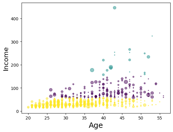
Kesimpulan
Dari datset diatas, kita dapat membuat 3 cluster, dengan segmentasi sebagai berikut:
- Kuning : dewasa muda, pendapatan rendah
- Ungu: dewasa menengah, pendapatan kelas menengah
- Hijau: dewasa tua, pendapatan tinggi